Correlations

Identifying correlations between assets in financial markets is vital in constructing diversified portfolios, managing risk, and improving returns. Correlation, in its simplest form, measures the relationship between two assets and how they move respectively to each other. A high positive correlation suggests that the assets tend to move in the same direction, while a negative correlation indicates that they often move in opposite directions. Recognising these relationships is essential for quantitative analysts and portfolio managers alike, as it informs decisions about risk management and asset allocation.

Identifying correlations between assets

Diversification is a well-known strategy to reduce risk in investment portfolios. The idea is to combine assets that are not highly correlated or ideally negatively correlated so that gains in another can offset losses in one asset. This approach reduces portfolio volatility and can enhance the overall risk-adjusted returns. For example, a portfolio that includes both stocks and bonds might benefit during economic downturns, as bonds typically perform better when equities underperform. Identifying correlations helps us to understand these dynamics, avoid overexposure to similarly behaving assets, and find opportunities for diversification.

Calculating correlations

Correlation is most commonly measured using the Pearson correlation coefficient, which ranges from -1 to +1 in the analysis of financial markets. +1 signifies a perfect positive correlation, 0 indicates no linear relationship, and -1 reflects a perfect negative correlation.

In this instance, we calculate the Pearson correlation between the close prices of each rotation of different financial assets over specific time intervals. For two time series, X (e.g., prices of asset A) and Y (prices of asset B), the correlation coefficient r is calculated as:

Where:

• Xi and Yi are individual price observations,
• Bar{X} and Bar{Y} are the respective means of the two assets’ prices.

This equation standardises the covariance between the two assets by dividing it by the product of their standard deviations, ensuring that the resulting correlation lies between -1 and 1.

Asset classes included in the analysis

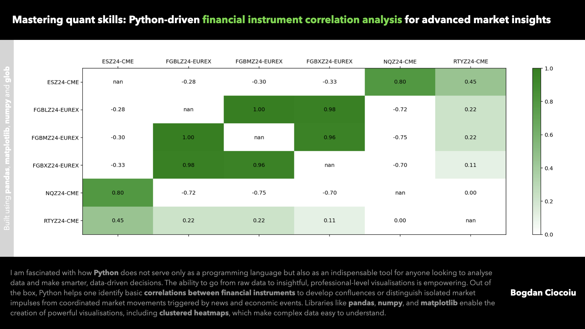
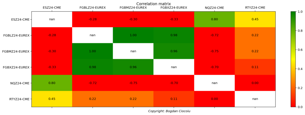
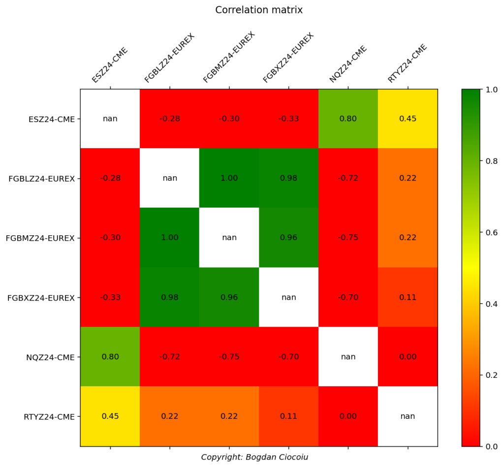
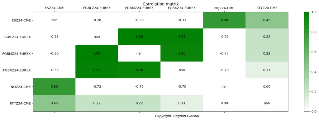
For this analysis, we examine the correlations between six prominent futures contracts: ES (S&P 500 E-mini), FGBL (Euro-Bund), FGBM (Euro-Bobl), FGBX (Euro-Schatz), NQ (Nasdaq-100 E-mini), and RTY (Russell 2000 E-mini). These assets represent different asset classes:

• Equities: ES, NQ, and RTY are equity index futures that track broad market indices.
• Government Bonds: FGBL, FGBM, and FGBX are German government bond futures of varying maturities.

The inclusion of these assets allows us to explore the relationships between equities and fixed-income securities, which often exhibit low or negative correlations. This provides insight into cross-asset diversification.

The interval and rotation period

Each dataset contains one-minute interval price data, meaning that the close price of each asset is recorded every minute during the trading day. The data sets focus on the last 100 rotations (i.e., the last 100 minutes). In this case, we analyse data rotated every minute, capturing real-time correlations that can evolve as market conditions change.

The minute-level data allows for a high-resolution view of price movements and how assets interact in short timeframes. This approach is beneficial for intraday trading strategies, where understanding minute-by-minute correlations can help traders execute profitable trades based on co-movements or divergences between assets.

Further work and hypotheses

While this analysis focuses on identifying basic correlations between assets over short time intervals, there are several ways to extend this work for deeper insights. One possible extension is to analyse how correlations change during different market regimes. For example, correlations between equities and bonds often shift during times of market stress (such as financial crises) compared to periods of calm. A regime-switching model could be employed to detect these shifts, which would help traders anticipate how asset relationships might evolve under different market conditions.

Another extension involves lead-lag relationships. Rather than simply examining contemporaneous correlations, one could investigate whether movements in one asset tend to lead to movements in another. This investigation could inform predictive models, providing signals for future price movements in one asset based on earlier movements in another.

Finally, incorporating volatility into the analysis could add further value. Assets may show varying correlations during periods of high or low volatility, and by applying models such as the dynamic conditional correlation (DCC) model, we could capture the time-varying nature of these relationships.

Identifying and understanding correlations between assets is crucial for managing risk and enhancing returns. By analysing these relationships at a granular level and extending the analysis to account for different market conditions, traders and portfolio managers can make more informed decisions in the ever-complex financial markets.