Time series analysis

Understanding time series data is crucial for making informed investment decisions in financial markets and the quantum analysis space. Time series analysis allows financial professionals to model and forecast market movements, identify trends, and detect underlying patterns in asset prices, trading volumes, and economic indicators.

For quantitative analysts, the ability to apply robust statistical models to financial time series is essential in crafting trading strategies, risk management techniques, and portfolio optimisations. With the increase in available market data and the rise of algorithmic trading, mastering time series analysis has become a core skill for anyone looking to advance in the finance industry.

Application of the ARIMA model

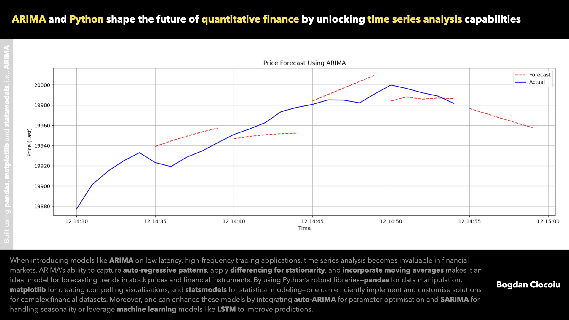
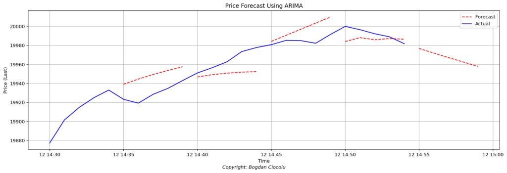
One of the most widely used models for time series analysis in finance is the ARIMA (AutoRegressive Integrated Moving Average) model. ARIMA is particularly well-suited to forecasting based on historical data, making it ideal for predicting asset prices, stock returns, or trading volumes over time. The model captures the inherent relationships within the time series, such as the dependency of future values on past observations (auto-regression), trends (integration), and random shocks (moving averages). By integrating these components, ARIMA provides a flexible tool for quantifying and forecasting future price movements.

In practical terms, ARIMA forecasts short-to-medium-term trends. For example, in Python, the ARIMA model predicts future values for the price of a financial instrument based on historical data. This forecast allows traders and analysts to make data-driven predictions about where prices might head in the next few minutes.

Components of the ARIMA model

ARIMA is composed of three main components, represented by its parameters (p, d, q):

• p (AutoRegressive term): This parameter captures the relationship between an observation and several lagged observations. It represents how past values influence the current value.
• d (Differencing): This variable makes the time series stationary by removing trends. Stationarity is essential in time series analysis because most statistical models, including ARIMA, assume a constant mean and variance over time.
• q (Moving Average term): This captures the relationship between the current observation and past residuals (errors). It accounts for the noise and shocks in the data that influence future values.

In Python, if we set the parameters as ARIMA(1, 1, 1), we use one autoregressive term (p=1), apply first-order differencing to make the data stationary (d=1), and use one lagged error term in the moving average (q=1).

Improving the application of ARIMA

While ARIMA is powerful, one can improve it further by automating the parameter selection process using tools such as auto-ARIMA. This ensures the best possible model configuration is selected based on the data. Moreover, adding exogenous variables (ARIMAX) such as trading volumes, interest rates, or macroeconomic indicators can improve the model’s predictive power. Handling seasonality more explicitly with models like SARIMA is another approach, especially for data with clear seasonal patterns (e.g., quarterly earnings or monthly sales figures).

Libraries used in the generated plot

In Python, several powerful libraries handle data manipulation, statistical modelling, and plotting:

1. pandas: A powerful library for data manipulation and analysis. It is used here to read and handle time series data from a file.
2. matplotlib: A comprehensive library for creating static, animated, and interactive visualisations in Python. It is used in this script to plot actual and forecasted prices.
3. statsmodels: This library provides classes and functions for estimating and testing statistical models. The ARIMA model is provided by statsmodels.tsa.arima.model.

Extending the work for more insights

This analysis could be further extended by exploring more advanced time series models, such as GARCH (Generalized Autoregressive Conditional Heteroskedasticity), commonly used to model financial volatility. Machine learning models like Long Short-Term Memory (LSTM) neural networks could also improve forecasting accuracy, especially for more complex and non-linear data.

Exploring multi-variate time series models that consider the relationships between multiple assets or economic indicators could provide deeper insights into market behaviour. This type of analysis helps uncover correlations, causations, and opportunities for arbitrage in financial markets.

Mastering time series analysis and applying models like ARIMA are essential skills for quantitative analysts in finance. By leveraging Python’s vast ecosystem of libraries, analysts can efficiently process financial data, develop accurate models, and generate valuable insights for decision-making.